Marking telomeres on a simple ideogram in R
How to make a basic telomere-marked ideogram using just ggplot2.
This article is part of our technical series, designed to provide the bioscience community with in-depth knowledge and insight from experts working at the Earlham Institute.
I was recently running the telomere identifier Tapestry on some genome assemblies to assess how close they were to chromosome-level. Tapestry already outputs an ideogram of assembly scaffolds marked with telomeres, but I wanted to customise the plot to make it clearer when showing collaborators.
There are a couple of R packages that can produce ideograms, including karyoploteR and ggbio, both of which I’ve dabbled in. But in this case I really wanted something even simpler than what either of those packages offer, and instead made a very basic telomere-marked ideogram using just ggplot2.
Dr Rowena Hill is a Postdoctoral Research Scientist at the Earlham Institute, studying the genome of the wheat root pathogen take-all, as part of the Delivering Sustainable Wheat (DSW) programme.
Rowena gained a PhD at the Royal Botanic Gardens, Kew and Queen Mary University of London, focusing on the diversity and evolution of fungi and plant-fungal interactions.
For the absolute simplest plot, the tsv produced during a Tapestry run contains all the information needed.
#Read in tapestry output file
tapestry <- read.csv("contig_details.tsv", sep="\t")
library(tidyverse)
tapestry %>%
  select(Contig, Length, GC., StartTelomeres, EndTelomeres) %>%
  slice_head(n=10)
##       Contig  Length  GC. StartTelomeres EndTelomeres
## 1 scaffold_1 7084357 51.3              0           18
## 2 scaffold_2 6698278 51.1             20           20
## 3 scaffold_3 6429383 50.1              0           18
## 4 scaffold_4 5545257 51.1              2            0
## 5 scaffold_5 3905873 50.3              0           13
## 6 scaffold_6 3299090 50.9             21           17
## 7 scaffold_7 1474513 49.5             22            0
## 8 scaffold_8  834656 48.0             16            6
## 9 scaffold_9   21427 32.6              0            1
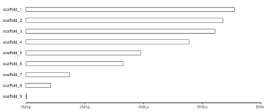
We can then use 'geom_rect' to plot the scaffolds.
#Make sure the scaffolds are ordered from largest to smallest for
#plotting
tapestry$Contig <- factor(
  tapestry$Contig,
  levels=tapestry$Contig[order(tapestry$Length, decreasing=FALSE)]
)
library(ggplot2)
library(scales)
library(tgutil)
#Plot ideograms
gg.ideogram <- ggplot(tapestry, aes(x=Contig, y=Length)) +
  geom_rect(aes(ymax=Length),
            ymin=1,
            xmin=as.numeric(tapestry$Contig)-0.2,
            xmax=as.numeric(tapestry$Contig)+0.2,
            fill="white",
            colour="dimgrey") +
  scale_y_continuous(
    limits=c(0, ceiling(max(tapestry$Length)/1e6)*1e6),
    labels=label_number(
      accuracy=1,
      scale=1e-6,
      suffix="Mbp"),
    expand=c(0, 100)
  ) +
  coord_flip(clip="off") +
  theme(axis.text.y=element_text(
    colour="black",
    size=8,
    margin=margin(r=5)
  ),
  axis.text.x=element_text(size=8),
  axis.ticks.y=element_blank(),
  axis.title=element_blank(),
  axis.line.x=element_line(),
  panel.grid.major=element_blank(),
  panel.grid.minor=element_blank(),
  panel.background=element_blank()) +
  ggpreview(width=7, height=3, units="in")
Now we need to make an additional dataframe with telomere positions.
#Restructure dataframe for plotting
telomeres <- tapestry %>%
  gather(telomere, num.telomeres, StartTelomeres, EndTelomeres)
#Replace 0 telomeres with NA
telomeres$num.telomeres[telomeres$num.telomeres == 0] <- NA
#Add positions for start and end of scaffolds
telomeres$y.pos <- ifelse(
  telomeres$telomere == "StartTelomeres", 1, telomeres$Length
)
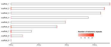
We can then add the telomeres to the scaffolds using 'geom_segment'.
#Add telomeres to ideogram
gg.ideogram.telomeres <- gg.ideogram +
  geom_segment(data=telomeres,
               aes(y=y.pos,
                   yend=y.pos,
                   colour=num.telomeres),
               x=as.numeric(telomeres$Contig)-0.3,
               xend=as.numeric(telomeres$Contig)+0.3,
               size=0.7) +
  scale_y_continuous(labels=label_number(accuracy=1,
                                         scale=1e-6,
                                         suffix="Mbp"),
                     expand=c(0, 100)) +
  scale_colour_gradient(
    name="Number of telomeric repeats",
    limits=c(1, max(na.omit(telomeres$num.telomeres))),
    low="#ffbdbd", high="#ff0000", na.value="transparent"
  ) +
  guides(colour=guide_colourbar(
    title.position="top",
    title.theme=element_text(face="bold", size=8))
  ) +
  theme(legend.position=c(0.8, 0.2),
        legend.direction="horizontal",
        legend.text=element_text(size=7),
        legend.key.size=unit(0.5, "cm"),
        legend.margin=margin(0, 0, 0, 0, unit="pt")) +
  ggpreview(width=7, height=3, units="in")
The plot produced by Tapestry colours telomeres opaque red if there are more than 20 repeats detected at the scaffold end, and semi-transparent if up to 20 are detected. Here I’ve opted to use a continuous gradient, but this could easily be modified depending on preference.
Alternatively, if we have already annotated the genome and want to further customise the ideogram, we can read in the gff3 file.
library(rtracklayer)
#Import the annotation
annotation <- import("Gnomoniopsis_smithogilvyi_IMI355082.gff3")
as.data.frame(annotation) %>%
  select(seqnames, start, end, type, ID, Name) %>%
  slice_head(n=10)
##      seqnames start   end type                    ID Name
## 1  scaffold_1 16179 17332 gene          N0V93_000001 <NA>
## 2  scaffold_1 16179 17332 mRNA       N0V93_000001-T1 <NA>
## 3  scaffold_1 16179 16744 exon N0V93_000001-T1.exon1 <NA>
## 4  scaffold_1 16851 17257 exon N0V93_000001-T1.exon2 <NA>
## 5  scaffold_1 17307 17332 exon N0V93_000001-T1.exon3 <NA>
## 6  scaffold_1 16179 16744  CDS   N0V93_000001-T1.cds <NA>
## 7  scaffold_1 16851 17257  CDS   N0V93_000001-T1.cds <NA>
## 8  scaffold_1 17307 17332  CDS   N0V93_000001-T1.cds <NA>
## 9  scaffold_1 18689 20177 gene          N0V93_000002 <NA>
## 10 scaffold_1 18689 20177 mRNA       N0V93_000002-T1 <NA>
For instance, we may want to only plot scaffolds which actually have gene models on them, and so can filter out the other scaffolds before plotting - in this case nothing changes as all our scaffolds have gene models on them!
#Filter out scaffolds with no annotated gene models
tapestry <-
  tapestry[tapestry$Contig %in% levels(seqnames(annotation)),]
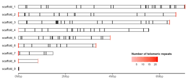
If we have the gff we can also add certain features to the ideogram.
#Make dataframe with start and end positions for tRNAs
tRNAs <- as.data.frame(annotation) %>%
  filter(type == "tRNA") %>%
  mutate(seqnames=factor(seqnames, levels=levels(tapestry$Contig)))
#Add tRNA positions
gg.ideogram.telomeres.trnas <- gg.ideogram.telomeres +
  geom_rect(data=tRNAs,
            aes(ymin=start, ymax=end),
            fill="grey",
            colour="black",
            xmin=as.numeric(tRNAs$seqnames)-0.2,
            xmax=as.numeric(tRNAs$seqnames)+0.2,
            inherit.aes=FALSE) +
  ggpreview(width=7, height=3, units="in")
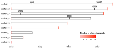
Or choose to highlight a specific genre.
#Make dataframe with start and end positions for RPB gene family members
genes <- as.data.frame(annotation) %>%
  filter(grepl("^RPB", Name)) %>%
  mutate(seqnames=factor(seqnames, levels=levels(tapestry$Contig)))
#Add gene positions with labels
gg.ideogram.telomeres.genes <- gg.ideogram.telomeres +
  geom_rect(data=genes,
            aes(ymin=start, ymax=end, fill=product),
            xmin=as.numeric(genes$seqnames)-0.2,
            xmax=as.numeric(genes$seqnames)+0.2,
            fill="grey",
            colour="black",
            inherit.aes=FALSE) +
  geom_label(data=genes,
             aes(label=Name, y=(start+end)/2),
             x=as.numeric(genes$seqnames)+0.5,
             label.size=NA,
             fontface="bold",
             fill="dimgrey",
             colour="white",
             size=2,
             label.padding=unit(2, "pt"),
             inherit.aes=FALSE) +
  ggpreview(width=7, height=3, units="in")
Of course, with all the excellent ggplot functions out there the sky’s the limit for how you could choose to customise these plots!
## R version 4.2.2 (2022-10-31 ucrt)
## Platform: x86_64-w64-mingw32/x64 (64-bit)
## Running under: Windows 10 x64 (build 22621)
##
## Matrix products: default
##
## locale:
## [1] LC_COLLATE=English_United Kingdom.utf8
## [2] LC_CTYPE=English_United Kingdom.utf8
## [3] LC_MONETARY=English_United Kingdom.utf8
## [4] LC_NUMERIC=C
## [5] LC_TIME=English_United Kingdom.utf8
##
## attached base packages:
## [1] stats4    stats     graphics  grDevices utils     datasets  methods
## [8] base
##
## other attached packages:
##  [1] rtracklayer_1.58.0   GenomicRanges_1.50.2 GenomeInfoDb_1.34.9
##  [4] IRanges_2.32.0       S4Vectors_0.36.2     BiocGenerics_0.44.0
##  [7] tgutil_0.1.14        scales_1.2.1         forcats_0.5.2
## [10] stringr_1.5.0        dplyr_1.0.10         purrr_1.0.1
## [13] readr_2.1.3          tidyr_1.2.1          tibble_3.1.8
## [16] ggplot2_3.4.0        tidyverse_1.3.2
##
## loaded via a namespace (and not attached):
##  [1] matrixStats_0.63.0          bitops_1.0-7
##  [3] fs_1.5.2                    lubridate_1.9.0
##  [5] httr_1.4.4                  tools_4.2.2
##  [7] backports_1.4.1             utf8_1.2.2
##  [9] R6_2.5.1                    DBI_1.1.3
## [11] colorspace_2.0-3            withr_2.5.0
## [13] tidyselect_1.2.0            compiler_4.2.2
## [15] Biobase_2.58.0              textshaping_0.3.6
## [17] cli_3.6.0                   rvest_1.0.3
## [19] xml2_1.3.3                  DelayedArray_0.23.2
## [21] labeling_0.4.2              systemfonts_1.0.4
## [23] digest_0.6.31               Rsamtools_2.14.0
## [25] rmarkdown_2.19              XVector_0.38.0
## [27] pkgconfig_2.0.3             htmltools_0.5.4
## [29] MatrixGenerics_1.10.0       dbplyr_2.3.0
## [31] fastmap_1.1.0               highr_0.10
## [33] rlang_1.0.6                 readxl_1.4.1
## [35] rstudioapi_0.14             BiocIO_1.8.0
## [37] farver_2.1.1                generics_0.1.3
## [39] jsonlite_1.8.4              BiocParallel_1.32.5
## [41] googlesheets4_1.0.1         RCurl_1.98-1.10
## [43] magrittr_2.0.3              GenomeInfoDbData_1.2.9
## [45] Matrix_1.5-1                munsell_0.5.0
## [47] fansi_1.0.3                 lifecycle_1.0.3
## [49] stringi_1.7.12              yaml_2.3.6
## [51] SummarizedExperiment_1.28.0 zlibbioc_1.44.0
## [53] grid_4.2.2                  parallel_4.2.2
## [55] crayon_1.5.2                lattice_0.20-45
## [57] Biostrings_2.66.0           haven_2.5.1
## [59] hms_1.1.2                   knitr_1.41
## [61] pillar_1.8.1                rjson_0.2.21
## [63] codetools_0.2-18            reprex_2.0.2
## [65] XML_3.99-0.13               glue_1.6.2
## [67] evaluate_0.19               modelr_0.1.10
## [69] png_0.1-8                   vctrs_0.5.1
## [71] tzdb_0.3.0                  cellranger_1.1.0
## [73] gtable_0.3.1                assertthat_0.2.1
## [75] xfun_0.36                   broom_1.0.2
## [77] restfulr_0.0.15             ragg_1.2.5
## [79] googledrive_2.0.0           gargle_1.2.1
## [81] GenomicAlignments_1.34.0    timechange_0.2.0
## [83] ellipsis_0.3.2