Plotting phylogenetic trees in R: alternating clade highlights
A guide to highlighting clades in phylogenetic trees in R
This article is part of our technical series, designed to provide the bioscience community with in-depth knowledge and insight from experts working at the Earlham Institute.
If you’ve dipped a toe into plotting phylogenetic trees before, you will likely be aware of the R package ggtree. For even the most niche customisations, I’ve yet to encounter something that I couldn’t somehow manage to do with the help of ggtree.
There’s already plenty of documentation out there for how to use ggtree, but there is the odd thing I come up against that I haven’t seen explicitly demonstrated before.
Here I’ll show how I highlight clades in my trees – probably the most fundamental customisation that anybody wants to be able to do – but without having to manually trawl through figuring out which nodes are associated with which clades.
Dr Rowena Hill is a Postdoctoral Research Scientist at the Earlham Institute, studying the genome of the wheat root pathogen take-all, as part of the Delivering Sustainable Wheat (DSW) programme.
Rowena gained a PhD at the Royal Botanic Gardens, Kew and Queen Mary University of London, focusing on the diversity and evolution of fungi and plant-fungal interactions.
In this example I’m going to use the tree and metadata from my recent paper in Molecular Biology and Evolution, which can be downloaded from my Github page.
This is an unrooted tree, so first we’ll root it with the outgroup.
library(ape)
#Read in tree
tree <- read.tree("fus_proteins_62T.raxml.support")
#Root tree
tree <- root(tree, "Ilysp1_GeneCatalog_proteins_20121116",
             resolve.root=TRUE, edgelabel=TRUE)
tree
##
## Phylogenetic tree with 62 tips and 61 internal nodes.
##
## Tip labels:
## GCA_013396075.1_ASM1339607v1_protein, fusotu1.proteins, fusotu3.proteins, GCA_900044065.1_Genome_assembly_version_1_protein, fusotu7.proteins, GCA_900067095.1_F._proliferatum_ET1_version_1_protein, ...
## Node labels:
## Root, 100, 100, 100, 100, 100, ...
##
## Rooted; includes branch lengths.##
## Phylogenetic tree with 62 tips and 61 internal nodes.
##
## Tip labels:
## GCA_013396075.1_ASM1339607v1_protein, fusotu1.proteins, fusotu3.proteins, GCA_900044065.1_Genome_assembly_version_1_protein, fusotu7.proteins, GCA_900067095.1_F._proliferatum_ET1_version_1_protein, ...
## Node labels:
## Root, 100, 100, 100, 100, 100, ...
##
## Rooted; includes branch lengths.
Now we can plot it very simply with tip labels to see what we’re working with.
library(ggtree)
ggtree(tree, linewidth=0.5) +
  xlim(0, 0.5) +
  geom_tiplab(size=2)
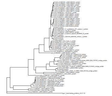
In order to customise this plot, we can attach a dataframe containing metadata to the tree object - just make sure that the exact tip labels in the tree are in the first column of the dataframe.
#Read in metadata
metadata <- read.csv("fus_62T_metadata.csv")
head(metadata)
##                                  label                     name          sc
## 1 GCA_012931995.1_ASM1293199v1_protein Albonectria albosuccinea Albonectria
## 2 GCA_013266205.1_ASM1326620v1_protein Albonectria rigidiuscula Albonectria
## 3  GCA_002980475.2_ASM298047v2_protein      Fusarium beomiforme   burgessii
## 4 GCA_012932025.1_ASM1293202v1_protein Fusarium austroafricanum    concolor
## 5 GCA_012932015.1_ASM1293201v1_protein        Fusarium acutatum   fujikuroi
## 6  GCA_001654555.2_ASM165455v2_protein       Fusarium agapanthi   fujikuroi
##   sc.abb
## 1    Alb
## 2    Alb
## 3  FBRSC
## 4  FCOSC
## 5   FFSC
## 6   FFSC
This allows us to add more informative tip labels.
ggtree(tree, linewidth=0.5) %<+% metadata +
  xlim(0, 0.4) +
  geom_tiplab(aes(label=name), size=2)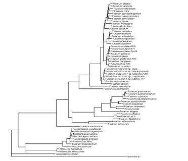
Here we want to highlight clades belonging to different genera or species complexes, which we have information for in our metadata dataframe.
To do this, we can make use of the ape function 'MRCA', which finds the most recent common ancestor, i.e. node, for a given set of tips in a tree.
#Make dataframe for clade nodes
clades.df <- data.frame(
  clade=unique(metadata$sc.abb),
  node=NA
)
#Find the most recent common ancestor for each clade
for (i in 1:length(clades.df$clade)) {

  clades.df$node[i] <- MRCA(
    tree,
    metadata$label[metadata$sc.abb == clades.df$clade[i]]
    )

}
Now we can simply use the dataframe of MRCA nodes to inform our highlights. Note that I am choosing to start with a blank tree, then adding the highlights before plotting the tree and tips last, as the order in which you add layers in a ggplot matters and I don’t want my highlights to block out the other layers.
#Add highlights
gg.tree <- ggtree(tree, linetype=NA) %<+% metadata +
  geom_highlight(data=clades.df,
                 aes(node=node, fill=clade),
                 alpha=1,
                 align="right",
                 extend=0.1,
                 show.legend=FALSE) +
  geom_tree(linewidth=0.5) +
  xlim(0, 0.4) +
  geom_tiplab(aes(label=name), size=2)
gg.tree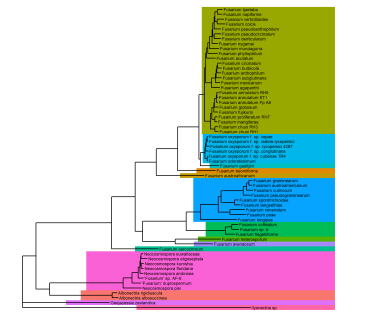
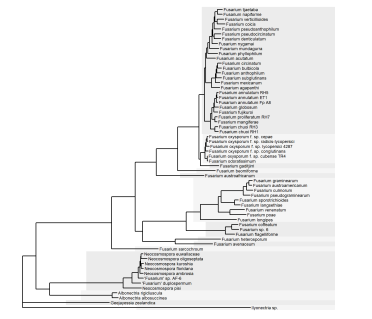
Instead of using different colours for every clade, you may just want to use highlights to make the distinctions between sister clades obvious.
If so, we can assign clades a binary value that alternates with the order that clades appear in the tree. An easy way to do this is by accessing the data from the ggtree object using 'gg.tree$data'.
library(dplyr)
#Order the clades dataframe to match the tree
clades.df <- clades.df[match(gg.tree$data %>%
                               filter(isTip == "TRUE") %>%
                               arrange(y) %>%
                               pull(sc.abb) %>%
                               unique(),
                             clades.df$clade),]
#Add column with alternating binary value
clades.df$highlight <- rep(c(0,1),
                           length.out=length(clades.df$clade))
head(clades.df)
##       clade node highlight
## 14 outgroup   38         0
## 13      Gee   37         1
## 1       Alb  105         0
## 11      Neo   98         1
## 7      FLSC   26         0
## 12     FTSC   24         1
Now we can colour the highlights by the new binary value and give it our own manual colour scale.
#Add highlights
gg.tree <- ggtree(tree, linetype=NA) %<+% metadata +
  geom_highlight(data=clades.df,
                 aes(node=node, fill=as.factor(highlight)),
                 alpha=1,
                 align="right",
                 extend=0.1,
                 show.legend=FALSE) +
  geom_tree(linewidth=0.5) +
  xlim(0, 0.4) +
  geom_tiplab(aes(label=name), size=2) +
  scale_fill_manual(values=c("#F5F5F5", "#ECECEC"))
gg.tree
The exact same principle can be used to add clade labels too. At the time of writing, 'mapping=' needs to be explicitly used to assign the aes values, otherwise it throws an error.
#Add clade labels
gg.tree +
  geom_cladelab(data=clades.df,
                mapping=aes(node=node, label=clade),
                fontsize=2,
                align=TRUE,
                offset=0.1,
                offset.text=0.01)

And, with some tweaking of the extend and offset parameters, this works just the same for circular tree layouts.
ggtree(tree, layout="circular", linetype=NA) %<+% metadata +
  geom_highlight(data=clades.df,
                 aes(node=node, fill=as.factor(highlight)),
                 alpha=1,
                 align="right",
                 extend=0.04,
                 show.legend=FALSE) +
  geom_cladelab(data=clades.df,
                mapping=aes(node=node, label=clade),
                fontsize=2,
                align="TRUE",
                angle="auto",
                offset=0.04,
                offset.text=0.01) +
  geom_tree(linewidth=0.3) +
  geom_tippoint() +
  xlim(0, 0.35) +
  scale_fill_manual(values=c("#F5F5F5", "#ECECEC"))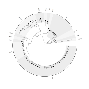
## R version 4.2.2 (2022-10-31 ucrt)
## Platform: x86_64-w64-mingw32/x64 (64-bit)
## Running under: Windows 10 x64 (build 22621)
##
## Matrix products: default
##
## locale:
## [1] LC_COLLATE=English_United Kingdom.utf8
## [2] LC_CTYPE=English_United Kingdom.utf8
## [3] LC_MONETARY=English_United Kingdom.utf8
## [4] LC_NUMERIC=C
## [5] LC_TIME=English_United Kingdom.utf8
##
## attached base packages:
## [1] stats     graphics  grDevices utils     datasets  methods   base
##
## other attached packages:
## [1] dplyr_1.1.2      ggtree_3.7.1.002 ape_5.7-1
##
## loaded via a namespace (and not attached):
##  [1] Rcpp_1.0.9         highr_0.10         pillar_1.9.0       compiler_4.2.2
##  [5] yulab.utils_0.0.6  tools_4.2.2        digest_0.6.31      aplot_0.1.10.011
##  [9] jsonlite_1.8.4     tidytree_0.4.2     evaluate_0.21      lifecycle_1.0.3
## [13] tibble_3.2.1       nlme_3.1-162       gtable_0.3.3       lattice_0.20-45
## [17] pkgconfig_2.0.3    rlang_1.1.1        cli_3.6.0          ggplotify_0.1.0
## [21] rstudioapi_0.14    patchwork_1.1.2    yaml_2.3.6         parallel_4.2.2
## [25] xfun_0.36          treeio_1.23.0      fastmap_1.1.0      gridExtra_2.3
## [29] withr_2.5.0        ggstar_1.0.4       knitr_1.42         gridGraphics_0.5-1
## [33] generics_0.1.3     vctrs_0.6.2        grid_4.2.2         tidyselect_1.2.0
## [37] glue_1.6.2         R6_2.5.1           fansi_1.0.3        rmarkdown_2.21
## [41] farver_2.1.1       purrr_1.0.1        tidyr_1.3.0        ggplot2_3.4.2
## [45] magrittr_2.0.3     scales_1.2.1       htmltools_0.5.4    colorspace_2.0-3
## [49] labeling_0.4.2     utf8_1.2.2         lazyeval_0.2.2     munsell_0.5.0
## [53] ggfun_0.1.1